(Subtle, Not At All Flashy)
Improvement to Photon Mapping
NeilFred Picciotto
In my project, I examined a particular aspect of photon mapping, and attempted to improve image quality in the case of relatively few photons being shot into the scene. In particular, I developed two extensions to PBRT's photon map integrator, and my results were fairly promising for the one scene I tested it on.
Goal
One of the parameters that the photon map integrator uses is the maxdist parameter; given a point p where a camera-ray intersected the scene, this parameter specifies the maximum distance from p that we will examine while looking for the k nearest photons, which we then use to estimate the irradiance at p. Put another way, as we grow a ball around p, attempting to enclose k photons, this is the maximum radius we allow the ball to reach before we give up and simply use however many photons have been enclosed at that point (even though it is fewer than k).
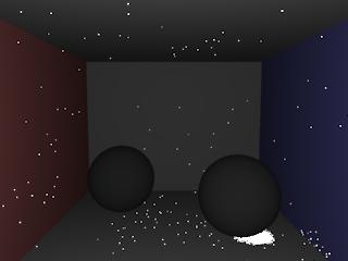
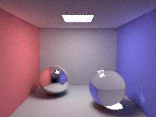
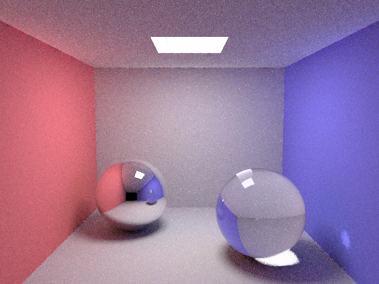
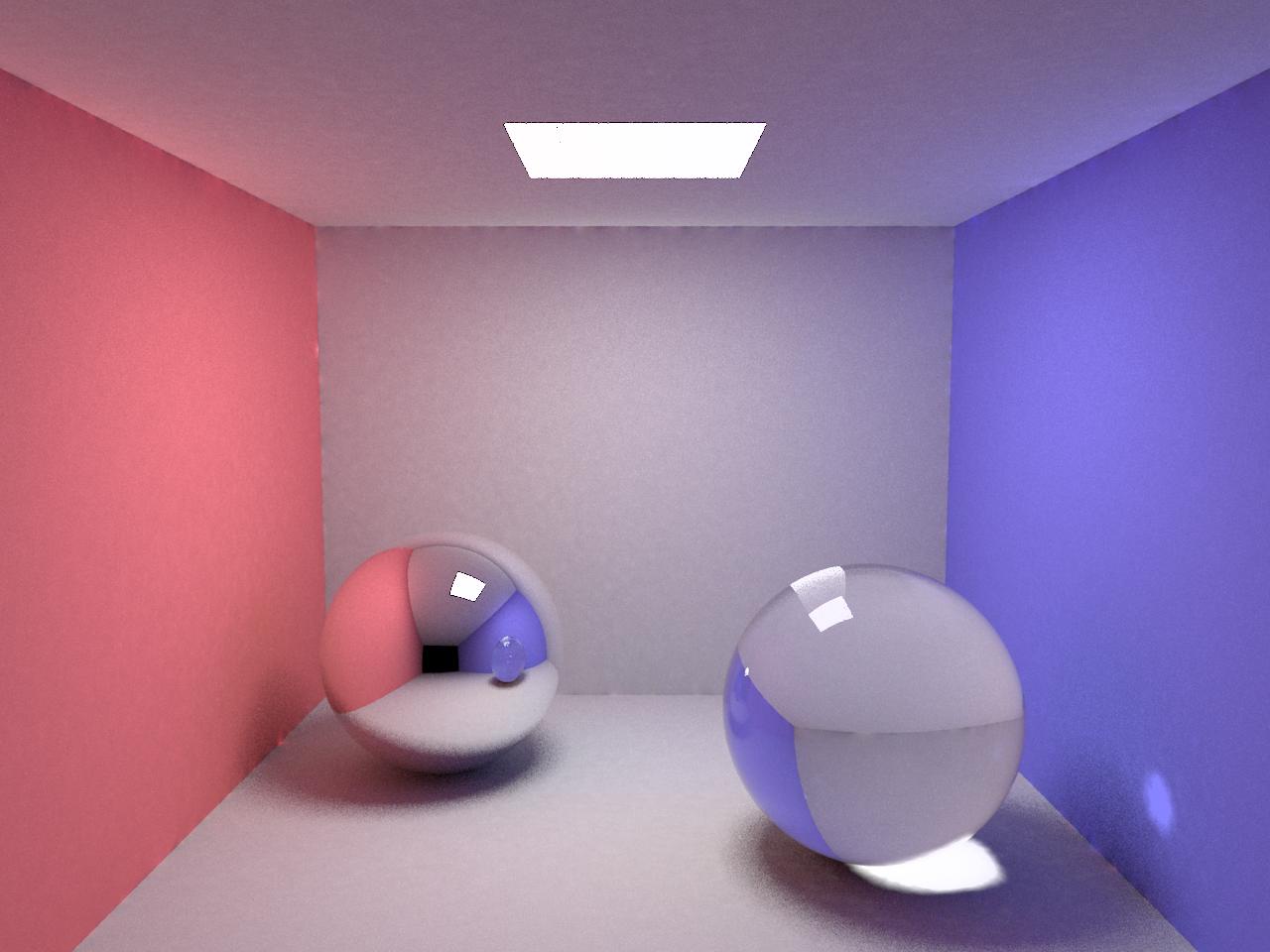
In this simple scene, and with 100,000 photons, we see the difference made by setting maxdist to 0.1 versus 1.0:
| 100,000 photons | |
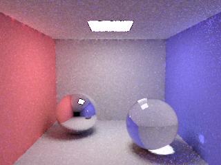 maximum photon distance = 0.1 (1m12s) |
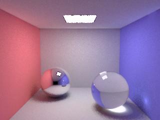 maximum photon distance = 1.0 (4m12s) |
(All rendering times reported are from rendering on one of the "myth" machines -- a 4-processor Intel Xeon 3.2 GHz machine with 1 GB of RAM.)
Note that in the image on the left, we get high-frequency noise on the walls due to too few samples (photons) being used to estimate irradiance. Whereas in the image on the right, those "speckles" have been blended together by using a larger ball size. However, that blending also has the effect of blurring out the caustic under the glass sphere, which, rendered correctly, should have sharp edges.
My goal was basically to try to achieve the "best of both worlds" -- to allow the photon map integrator to simultaneously render smooth walls and a sharp caustic, while still using only a small number of photons. Of course, that kind of improvement can be certainly be achieved with more photons in the scene:
| 5,000,000 photons | |
 maximum photon distance = 0.1 (14m56s) |
 maximum photon distance = 1.0 (25m18s) |
Note that because k (the desired number of photons) has remained fixed (at 100), with this much-more-dense set of photons, we generally find k of them within less than the 0.1 ball radius, and therefore we see that upping the maximum distance to 1.0 leads to almost exactly the same image, although it takes somewhat longer to render.
But again, I attempted to achieve a better image while still using only a small number of photons.
Sets of Photons
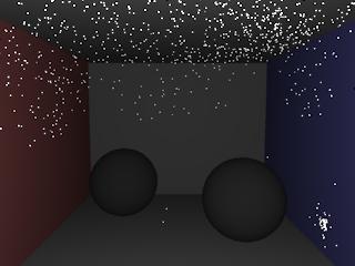
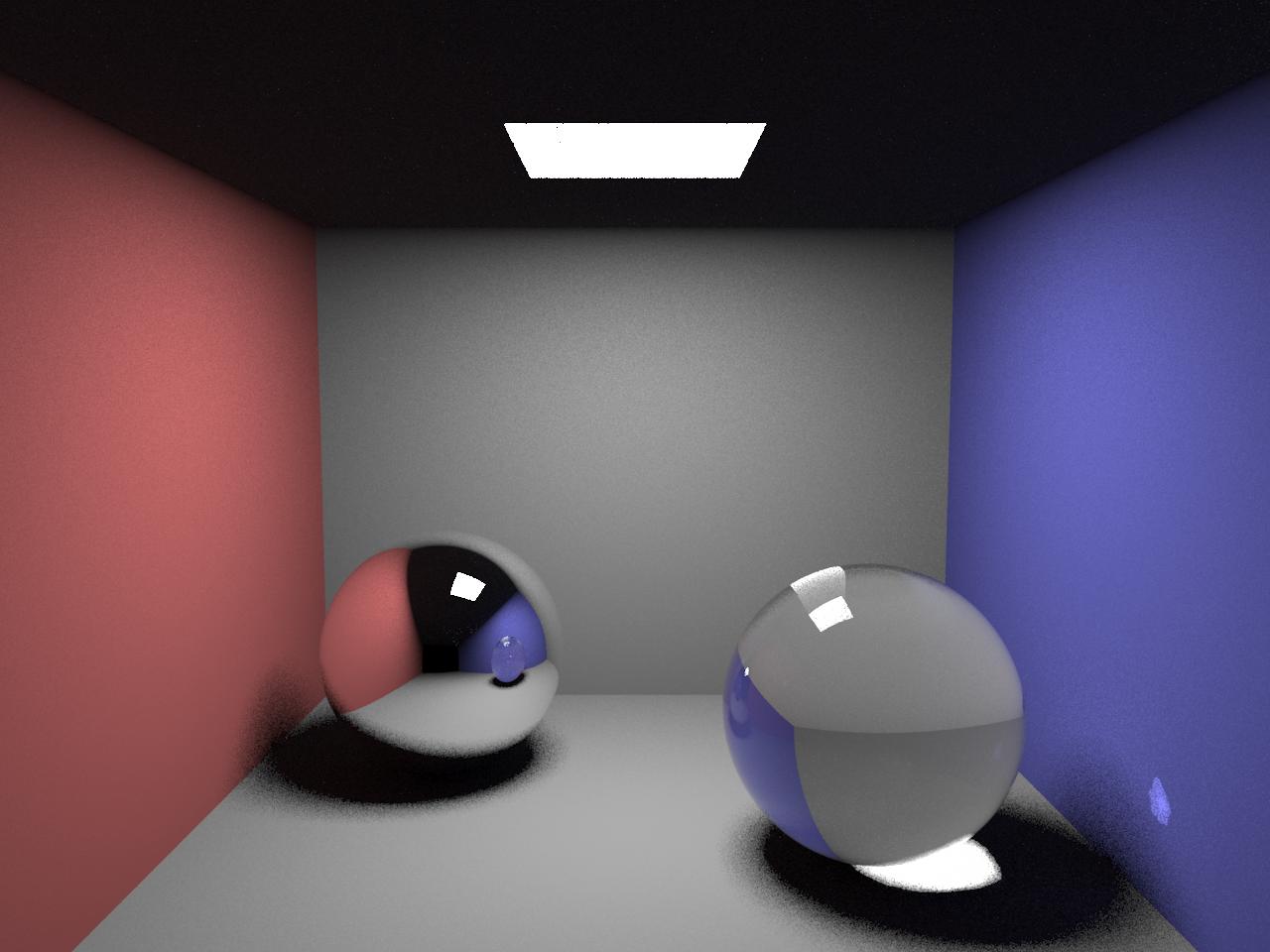
Let us now look at where the photons are. In the default PBRT implementation, photons are divided up into three categories: direct, indirect, and caustic, and a separate KD tree is maintained for each of these categories. On a run with just 50,000 photons, we can visualize these three sets of photons:
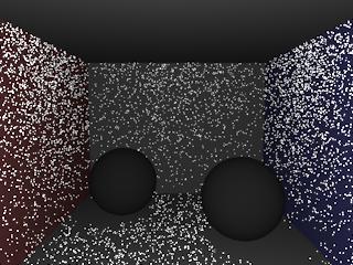 15,000 direct photons |
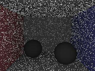 15,000 indirect photons |
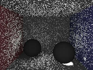 20,000 caustic photons | |
As we might expect, the direct photons are everywhere but on the ceiling and in the shadows of the two spheres, and the indirect photons are basically everywhere. The caustic photons are the interesting ones. Most notably, we see a high concentration under the glass sphere. But that sharp edge between those and the nearby ones is not going to be easy for the system to recognize as a sharp edge, without a lot of photons.
However, if we further sub-categorize the caustics based on their number of bounces, and maintain now six separate KD trees -- direct, indirect, and four for different numbers of caustics -- we get the following photon sets:
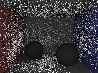 15,006 caustic photons (1 bounce) |
 3100 caustic photons (2 bounces) |
 1432 caustic photons (3 bounces) |
 462 caustic photons (4+ bounces) |
Here we see that the photons that have made just one bounce are mostly everywhere but in the shadow of the glass sphere. The caustic we're interested in under the glass sphere shows up among the 2-bounce photons (since transmission is considered a bounce -- the two bounces correspond to entering and then leaving the sphere), with relatively few spurious photons nearby. Among the 3-bounce photons we see the caustic on the wall (bounce off mirror, enter glass, leave glass). Note that with all the caustics together, that high-concentration region was less obvious. And then there are just a handful of 4-or-more-bounce photons.
So the key idea here is that by dividing the caustic photons up in this way, sharp edges will be easier to identify and correct for. Note that this idea of finer categorization is more general than just this simple use -- for example, if we had multiple light sources, it might also be helpful to divide up the direct photons based on which light source they originated from. The key fact being that identifying an edge between a bright region and a region with no light will always be simpler than between a bright region and a somewhat-less-bright region.
Along those lines, it's also worth noting that for the caustics, in a more complicated scene, merely counting the number of bounces might not be sufficient; we might actually want to track, for example, which object in the scene each bounce was associated with. Also note that indirect light -- almost by definition -- tends to be somewhat blurry and without sharp edges anyway, so finer subcategorization there is probably not worthwhile.
Uniformity of Photon Density
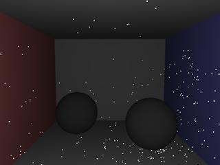
The next key observation is that uniformity of photon density in a region is the major property which distinguishes situations where the small ball does better from those where the large ball does better. Specifically, in those original two images:
|
small ball best when photon density is varying |
large ball best when photon density is uniform |
The small ball size does well for the edges of the caustic in the image on the left because the density of photons is changing a lot there; whereas the large ball does well on the walls and ceiling in the image on the right because the density of photons is fairly uniform there.
So we would like to find a way to detect that difference. I tried a number of things which didn't work very well before finally hitting upon a technique that actually seems to achieve the desired result reasonably well.
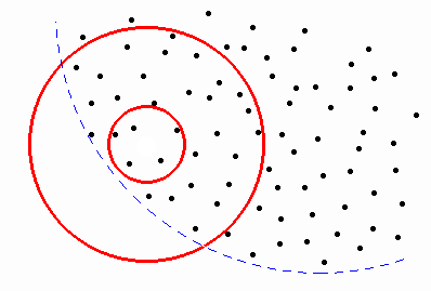
The key insight was to compute, based on the number of photons in the large ball, the expected number of photons for the small ball. Consider the following examples, where the dashed blue line indicates a sharp edge of light in the actual underlying scene:
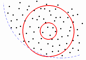
Here we see that the small ball and large ball have approximately equal density, so we choose the large ball for our computation here.
As we approach the edge, the density of photons within the small ball remains approximately constant, but as the large ball encloses some of the dark side of the boundary, its density goes down, so expected number of photons in the small ball goes down. Specifically, when the small ball contains more than twice as many photons as expected, we choose it instead of the large one.
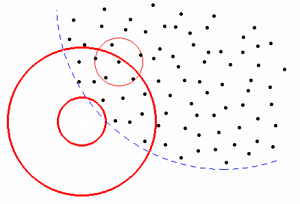
On the other side of the boundary, the small ball contains much fewer than the expected number of photons. In particular, when it contains fewer than half as many as expected, we make a second check. We consider the furthest photon within the large ball, and count the photons in a small ball around it: if the photons are high-density (more than twice expected) in that ball, we choose the low-density small ball.
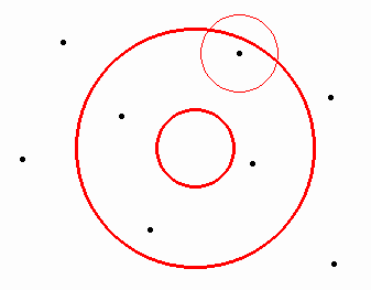
To see why we make that secondary check, consider now a relatively sparse area. Here, we might find that the small ball has fewer than half the expected number of photons, but since the small ball around the furthest photon is not high-density (it is perhaps approximately the expected density), we still choose the large ball.
Results
Combining these two techniques, we find that indeed, we are able to simultaneously achieve smooth walls and a sharp caustic, at the cost of some extra computation time.
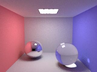
For comparison, we again present the original images:
| original (100,000 photons) | |
|
maximum photon distance = 0.1 (1m12s) |
maximum photon distance = 1.0 (4m12s) |
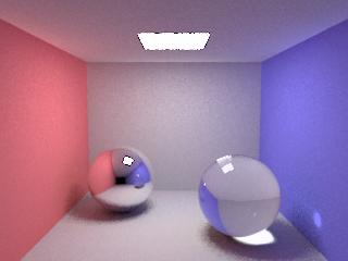
| my version (100,000 photons) | |
 small ball 0.1 / large ball 1.0 (5m20s) | |
Although the image quality obtained is certainly not as high as with more photons, it does achieve the goal of culling most of the good aspects of the two different images generated by the same number of photons.
It should be noted, however, that this improvement comes with a nontrivial cost in computation time. Basically, we wind up spending about the time of each of the two methods on its own. And indeed, a few simple tests suggested that for equal time, you get better results from the standard technique with more photons. However, the running time of my technique could certainly be considerably improved with a little optimization. For example, my code currently makes up to three separate lookups in the same KD tree for every one call made by the standard technique; and those first two lookups even use the same center point, and so we are effectively performing part of that walk twice, and hence some considerable speedup should be possible there. Furthermore, the third lookup is centered at a point which we have already found in the KD tree, so while the walk around that point is still required, the initial search to find that point could be avoided.
Even with such optimizations, of course, the running time clearly must always be at least somewhat worse than achieved without this technique, simply because more computation must be done. However, even if better results can always be obtained by using more photons, the memory footprint must also scale up as more photons are used. So if for a super-high-resolution image, say, you were already using the maximal number of photons your hardware could manage to hold in memory without resorting to constant page-swapping -- in that situation, my technique should be able to provide better results without requiring more memory.
And finally, a few high-resolution images -- going up to 1280 by 960, using 10 times as many photons (1 million), dropping the maximum distances by a factor of 10 (to .01 and .1):
orig, maxdist .01, 1M photons (19m39s)
orig, maxdist .1, 1M photons (29m25s)
mine, .01 / .1, 1M photons (44m12s)
As before, the first one is grainy, the second is smooth but with a somewhat blurred edge to the caustic (though really not too bad), and mine gets a little of each. But unfortunately it fails to highlight my technique... I didn't get a chance to experiment with very many permutations of the parameters to find a good set. Oh well.
Conclusion
I've presented two simple modifications to the standard photon mapping technique, which together provide for slightly better results in certain situations. The key ideas are to use a finer categorization of the photons, and to vary the maximal ball size according to the arrangement of photons in the neighborhood.
Oh, and here's my code.