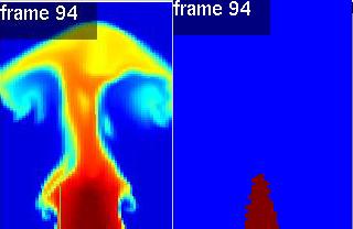
To model fire, I used Nguyen and Fedkiw's fire simulator introduced in Nguyen et.al. 2002 "Physically Based Modelling and Rendering of Fire." It simulates a two phase incompressible flow where one fluid is the fuel and one is the air. The interface between the two (the reaction surface) is represented as a dynamic level set. The pressure projection solver properly maintains the discontinuity of velocity and density. During each separate fluid's update the ghost fluid method is used to extrapolate to enforce the proper velocity jump conditions so that the fluid update can proceed directly. The parameters available include a flame speed in the normal direction, a curvature dependent flame speed component (which I set to zero for all applications), the position of sources, and the inflow velocity at sources. Additional turbulence was produced using vorticity confinement as introduced in Fedkiw et.al. 2001 "Visual Simulation of Smoke." The picture the near right depicts the temperature profile of a 2D simulation of fire whereas the far right depicts the levelset flame core.
The simulator outputs for each frame a density scalar field, temperature scalar field, and a levelset scalar field. In addition I augmented the solver to track massless marker particles for placing embers. The positions, temperatures, and velocities are stored for each particle. This preview(divx) shows the ember particles' motion.
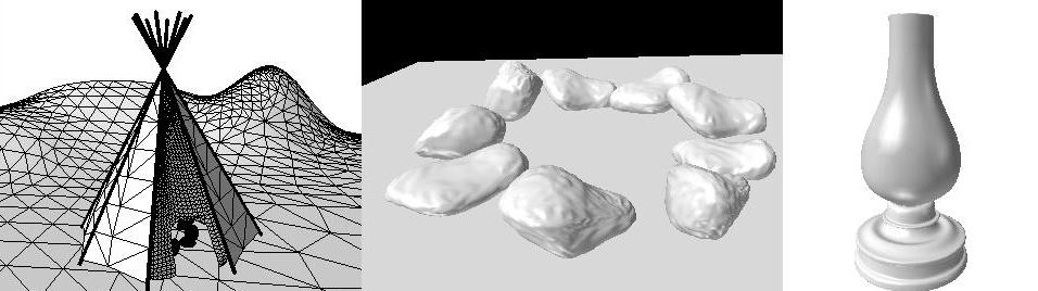
For the scene, I went through a bunch of different ideas. First, I thought maybe a lamp would be good, then a tepee with a fire. Finally a just settled on a campfire with rocks. I modeled all my scenes using maya and exported them to a triangulated surface format that my renderer supported. I finally settled on the rocks beecause of the simplicity. I modeled them using subidivision surfaces and added additional detail to the polygon representation by adding random perterbation in the normal direction. Below is a sampling of the scenes I produced:
 The first component that I
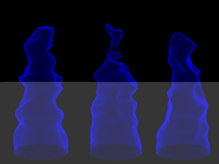
tried to model is the emissive blue core of the flame. The Nguyen paper mentions
this part of rendering but does not discuss how it should be accomplished. I
modeled the core as a thin blue emissive surface shader. I model it so that the
emission is brighter on grazing angles (where the ray would go through more of
the thin shell). So the brightness is inversely proportional to the dot product
of the normal with the ray direction. For photons that intersect the core I just
pass them on as the core is only emissive and doesn't absorb or scatter. Photons
are also emitted from the core to model the emission. The image on the right
depicts the blue core rendered. This movie(divx)
also shows it in motion.
The first component that I
tried to model is the emissive blue core of the flame. The Nguyen paper mentions
this part of rendering but does not discuss how it should be accomplished. I
modeled the core as a thin blue emissive surface shader. I model it so that the
emission is brighter on grazing angles (where the ray would go through more of
the thin shell). So the brightness is inversely proportional to the dot product
of the normal with the ray direction. For photons that intersect the core I just
pass them on as the core is only emissive and doesn't absorb or scatter. Photons
are also emitted from the core to model the emission. The image on the right
depicts the blue core rendered. This movie(divx)
also shows it in motion.
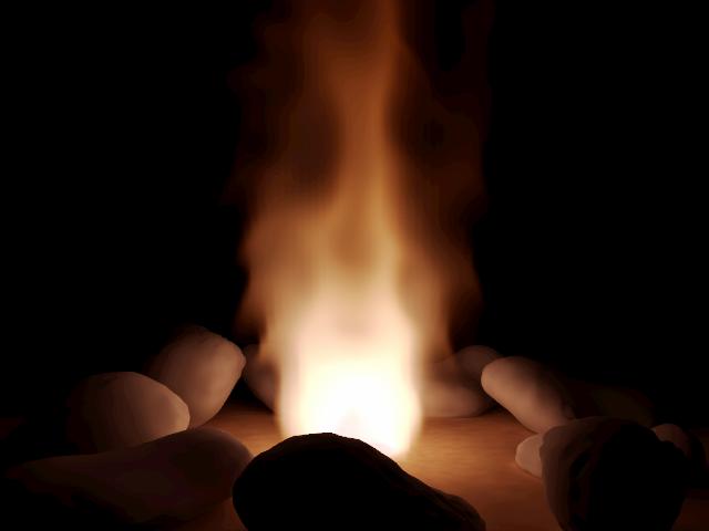
The major part of fire that we recognize is the orange-red look of the flames. This is caused by blackbody emission and the interaction with the gaseous products of the chemical oxidation. To capture this effect I follow the strategy outlines by Nguyen et.al. Namely, I solve the volume rendering equation through an emissive volume. The paper specifies taht they use monte carlo path tracing to capture the multiple scattering by during the forward (From eye ray trace) by importance sampling the Henyey-Greenstein phase function. I found that ignoring scattering completely and only accounting for absorption and emission produced very similar results to the paper. In fact, the smoke in the paper looks like it isn't scattering much. I integrate using a simple stochastic march through the volume. At each step we interpolate the temperature and density to get a value at the midpoint of the line segment. The density is used to drive the absorption coefficient (sigma_a) and the temperature is used to drive the emission. To obtain the emission radiance we need to take special care because of the high dynamic range perception issues of fire. I follow the strategy outlined in the paper where they use Planck's formula to find the blackbody emission spectrum given a temperature in kelvin. They then map this to XYZ and then LMS coordinates, scale to a whitepoint in LMS (set by the maximum temperature's blackbody emission) and convert to RGB. This RGB value is used for the volume integration emission. Undboutably a spectral volume simulation would be much more accurate, but their results (and mine) seem reasonable. I would like to try the spectral simulation in the future to see if it improves results significantly.
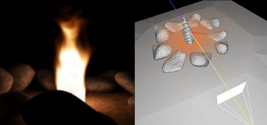
The paper unfortunately did not talk much about sampling the fire. This is probably the biggest unanswered question with figure (as well as other spatially varying volume light sources). I decided to use a relatively simple importance sampling scheme for photon emission. I construct a piecewise constant 3D PDF proportional to the viewer adjusted luminance given by the blackbody emission in that voxel. Then I construct the CDFs for the Pr(z|x,y), Pr(y|x) and Pr(x). Then, I can sample from these using the inversion method that we used for the infinite sphere lighting assignment. For photon emission we simply sample a position and direction. The position is given by the PDF sampling strategy. For the direction I use a isotropic scattering function so I simply choose randomly. Since I am using proper importance sampling I can emit each photon with the total power of the volume light source and the density estimation will give me the proper effect for free. Below the result of illuminating the rocks with the fire volume is shown below on the left. A visualization of the photons in the global map is shown in the image on the right.