My primary goal was to develop and implement a new algorithm or variation on an existing algorithm, implement one or more existing algorithms, and compare them. I also wanted to create a visualization of the algorithms. Lastly, I wanted to create a chess scene to show off my results.
My original project proposal can be found here .
The traditional algorithm searches out into the scene from one point on the film plane at a time and records the discovered scene points only at that one point. My algorithm uses the same approach to find visible points in the scene, but it handles them differently. It tries to project each discovered point back onto the film plane across its entire circle of confusion.
To achieve this, for each discovered point it takes additional samples of the aperture and considers the ray to the point in question from that spot on the aperture. If the point in the scene is visible along that ray, it finds the shading of the point from the point of view of the ray and traces the ray back to the image plane to find the point where that radiance should be recorded. If the point is not visible, the ray is discarded.
As a normalization, the weight of the radiance is divided by two factors: the number of samples made of the aperture and an estimate of the fraction of the aperture that can see the point. This can be thought of as dividing the weight of the probe that originally found the point by the expected number of locations on the image plane which will ultimately be affected by it.
A theoretical justification for the algorithm is worked out here . A point worth noting is that the theory is based on an approximation. This can be avoided, but the result will be messier. Also, the result is presumably biased. But, modulo the approximation error, the results will converge on the correct answer.
I wanted to get information to every pixel in the circle of confusion, so I chose the number of samples of the aperture to be the area of the circle of confusion measured in pixels. This does not guarantee that every pixel will be hit. Indeed, there are almost certainly more pixels intersected by the circle of confusion than its area. This is just a reasonable estimate. These samples are taken in a stratified way based on a coordinatization of the aperture using Shirley's mapping.
Misses of the scene are treated as hits on points infinitely far away having circles of confusion of the same size as the aperture. The rays from the lens to this point are all parallel to the original ray. Those that miss the scene are considered hits on the point at infinity and are recorded on the film. They have zero radiance and alpha values of zero. No shading need be done for them.
One could get a visibility factor estimate from the visibility tests that are already performed in the course of the algorithm, but this would require saving all the results until all the visibility test have been completed. To save space, I have implemented the visibility testing as a separate pass done at very low resolution in advance of the main work for the point.
To help compensate for this fact, the algorithm doesn't do all the work every time a point is discovered. As soon as a point is discovered, the algorithm knows its circle of confusion, which is a measure of the potential wastefulness of processing the point further. So the point is processed only with a probability inversely proportional to the area of its circle of confusion. This eliminates wastefulness and the need to divide by this factor.
More generally, it is the expected weight that must be divided by the two factors originally mentioned. So arbitrary factors can be shifted between the acceptance probability and the weight arbitrarily, as long as their product is the right thing.
The algorithm uses this to advantage in handling the background by giving it less processing at greater weight. It also takes advantage of the fact that visibility is computed in advance to reject points in the background that are fully visible more than points which are only partially visible. This heuristic helps distinguish parts of the background whose effects must be blended with those of the scene from those that are not relevant.
While the sampling of directions for shading should be increased to approach the correct solution in the limit, one of the versions of the algorithm that I have implemented simply uses one shading ray to process each scene point intersection. This is both for simplicity and to see how well the simplest approximation performs. Because the circles of confusion are flat shaded like spots, I call this the spots version. I call the original version the disks version to distinguish it from the spots version for lack of a better name.
The third version of my algorithm that I implemented simply combines a pass of the traditional algorithm with a pass of the spots version of my algorithm, allowing lrt to average the results. The spots version is faster, and the traditional algorithm has the potential to make up for the flat shading.
I implemented a stratified sampler to provide a good reference and also used that sampler to implement the disk and spots versions of my algorithm. I also implemented a probabilistic rejection version of the traditional algorithm. The initial results weren't promising, and, since I no longer found the idea compelling, I quickly dropped this algorithm from the project. I even implemented non-rejecting versions of my algorithm for completeness, but the theory and results here weren't compelling either, so they were also quickly dropped.
After observing the results, it occurred to me that the two techniques might well complement each other, so I implemented the hybrid version.
I wanted to compare the results between the algorithms using the same amount of computation. But stratified sampling doesn't adjust to a specified amount of computation, and it didn't seem fair to force my algorithms to adjust to fit computation that is just right for the stratified algorithm.
I came up with some interesting ideas about sequential sampling, but they are not fully developed and were not implemented, so they are not a part of the project.
In the end, I did run my algorithms sequentially against the computation used by the stratified algorithm. I chose to track the number of scene intersection tests as the measure of computation.
In order to have flexibility in when to stop the algorithm, computation needed to be broken up at a coarser level than even a single pixel. I implemented a dart-throwing sampler, which simply picks a random point anywhere on the film plane and one anywhere on the aperture for each sample. (Unlike the Poisson dart approach, samples are not rejected for being near other samples.) This coarseness makes for a far less regular algorithm than stratifying to a very fine level, so I also used this sampler with the traditional approach to serve as a more reasonable standard of comparison.
I compared five algorithm variations: stratified, dart (traditional with the dart sampler), disks, spots, and the hybrid version. For the hybrid version, one third of the computation went to the dart pass and two thirds went to the spots pass. This was a fairly arbitrary choice, with the idea being to use the dart pass to reinforce the spots pass.
The results for five amounts of computation are below, including tracked
statistics. The first picture of each set is stratified with some chosen number
of levels for the x and y subdivisions (shown first) and the lens coordinate
subdivisions (shown second). The remainder were run until they matched the
number of scene intersections of the stratified run. JPEG versions are shown,
which are links to the TIFF versions. At the end is a high-resolution stratified
picture.
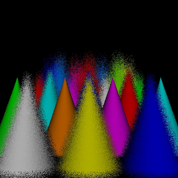
stratified: (1, 1, 1, 1).
Scene/Intersection Tests 360512
Scene/Point Shadings 360000
Camera/Eye
Rays Traced 360000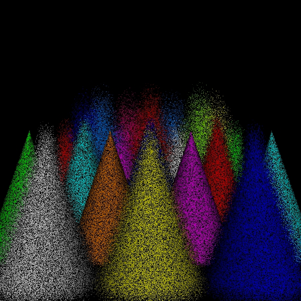
dart for 360000 intersect tests
Scene/Intersection Tests 360512
Scene/Point Shadings 360000
Camera/Eye
Rays Traced 360000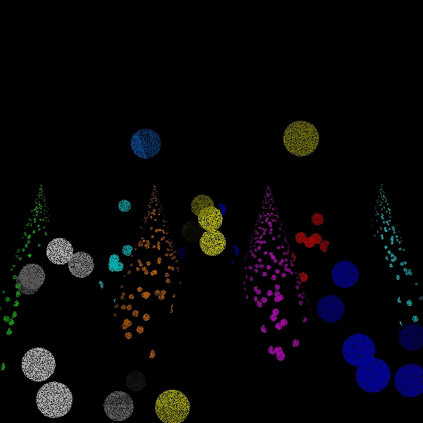
disks for 360000 intersect tests
Scene/Intersection Tests 367951
Scene/Point Shadings 39712
Camera/Eye
Rays Traced 83455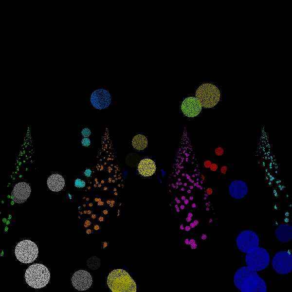
spots for 360000 intersect tests
Scene/Intersection Tests 360512
Scene/Point Shadings 916
Camera/Eye
Rays Traced 79664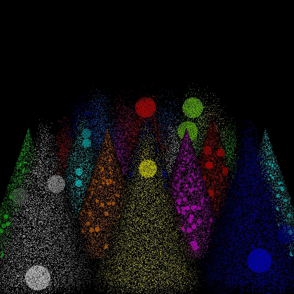
hybrid for 360000 intersect tests
Scene/Intersection Tests 367548
Scene/Point Shadings 120637
Camera/Eye
Rays Traced 175164

stratified: (1, 1, 2, 2).
Scene/Intersection Tests 1440512
Scene/Point Shadings
1440000
Camera/Eye Rays Traced 1440000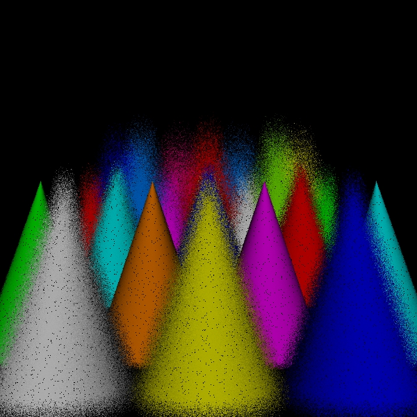
dart for 1440000 intersect tests
Scene/Intersection Tests 1440512
Scene/Point Shadings
1440000
Camera/Eye Rays Traced 1440000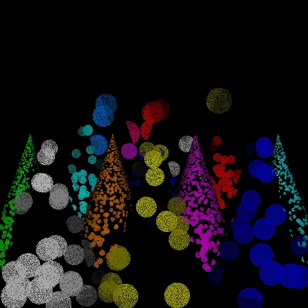
disks for 1440000 intersect tests
Scene/Intersection Tests 1440515
Scene/Point Shadings 139743
Camera/Eye
Rays Traced 319908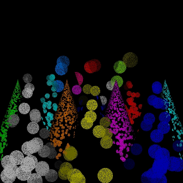
spots for 1440000 intersect tests
Scene/Intersection Tests 1440541
Scene/Point Shadings 3556
Camera/Eye
Rays Traced 327924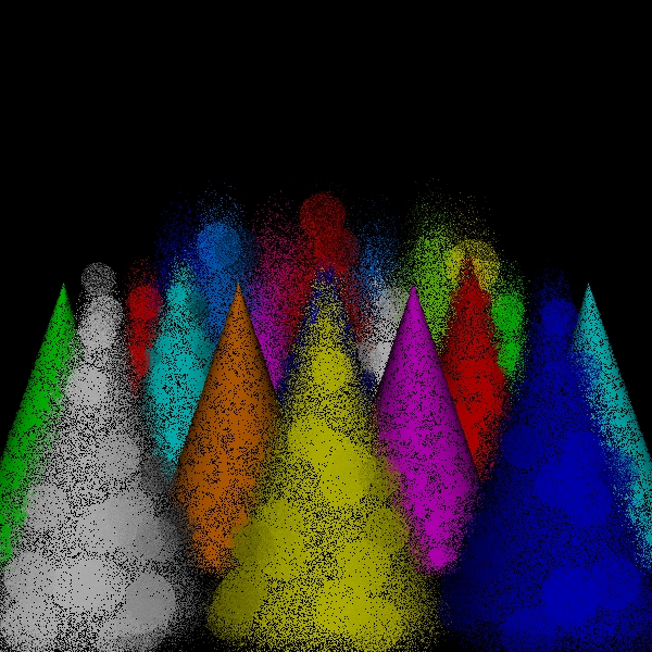
hybrid for 1440000 intersect tests
Scene/Intersection Tests 1440522
Scene/Point Shadings 482522
Camera/Eye
Rays Traced 719603

stratified: (2, 2, 2, 2).
Scene/Intersection Tests 5760512
Scene/Point Shadings
5760000
Camera/Eye Rays Traced 5760000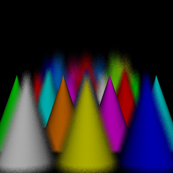
dart for 5760000 intersect tests
Scene/Intersection Tests 5760512
Scene/Point Shadings
5760000
Camera/Eye Rays Traced 5760000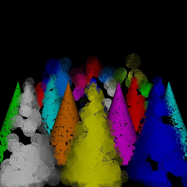
disks for 5760000 intersect tests
Scene/Intersection Tests 5760514
Scene/Point Shadings 687268
Camera/Eye
Rays Traced 1335525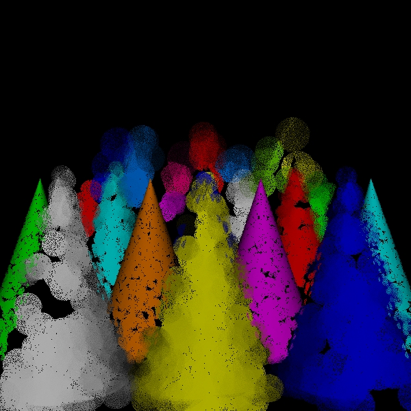
spots for 5760000 intersect tests
Scene/Intersection Tests 5760512
Scene/Point Shadings 14659
Camera/Eye
Rays Traced 1344876
hybrid for 5760000 intersect tests
Scene/Intersection Tests 5760515
Scene/Point Shadings
1929981
Camera/Eye Rays Traced 2826163

stratified: (3, 3, 3, 3).
Scene/Intersection Tests 29160512
Scene/Point Shadings
29160000
Camera/Eye Rays Traced 29160000
dart for 29160000 intersect tests
Scene/Intersection Tests 29160512
Scene/Point Shadings
29160000
Camera/Eye Rays Traced 29160000
disks for 29160000 intersect tests
Scene/Intersection Tests 29160514
Scene/Point Shadings
3636991
Camera/Eye Rays Traced 7012577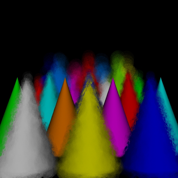
spots for 29160000 intersect tests
Scene/Intersection Tests 29160512
Scene/Point Shadings 77825
Camera/Eye
Rays Traced 7069968
hybrid for 29160000 intersect tests
Scene/Intersection Tests 29160512
Scene/Point Shadings
9772798
Camera/Eye Rays Traced 14527063

stratified: (5, 5, 5, 5).
Scene/Intersection Tests 225000512
Scene/Point Shadings
225000000
Camera/Eye Rays Traced 225000000
dart for 225000000 intersect tests
Scene/Intersection Tests 225000512
Scene/Point Shadings
225000000
Camera/Eye Rays Traced 225000000
disks for 225000000 intersect tests
Scene/Intersection Tests 225000512
Scene/Point Shadings
28284257
Camera/Eye Rays Traced 54767440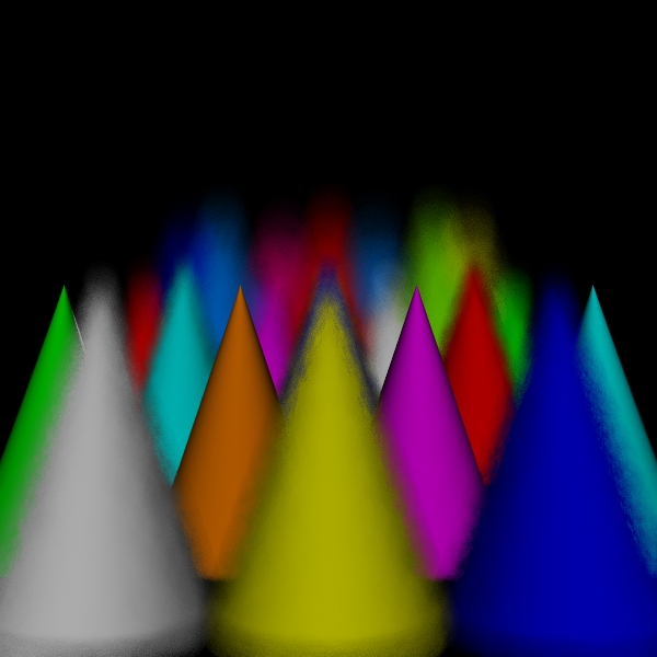
spots for 225000000 intersect tests
Scene/Intersection Tests 225000516
Scene/Point Shadings
603905
Camera/Eye Rays Traced 54998118
hybrid for 225000000 intersect tests
Scene/Intersection Tests 225000512
Scene/Point Shadings
75403186
Camera/Eye Rays Traced 111688554

stratified: (7, 7, 7, 7).
Scene/Intersection Tests 864360512
Scene/Point Shadings
864360000
Camera/Eye Rays Traced 864360000
The idea of trying to produce a coherent view is applicable in other domains, but I did not explore any of these. Motion blur is the most obvious. First, it is closely related. Second, people might be even more sensitive to whether they see the entire trajectory of an object than to whether they see the entire circle of confusion of an out-of-focus point.
I did not write a better integrator. My results are greatly limited by the fact that effects like blurry reflection are missing and that shading seems to be an unusually low fraction of the cost of dealing with a point found in the scene. A better scene would help here too.
I did not look into the effect of filters or relations to other issues such as aliasing.
I did not compare my algorithm against more sophisticated algorithms than stratification.
I did not create any visualization of the algorithms. Hopefully, the low-resolution pictures make the essence of the algorithms fairly clear.
My algorithm fares badly on the low end. It has overhead from probing the scene geometry which leaves it with little computation left for rendering. The algorithm could certainly do with improvements to reduce this overhead. Of course, the dart-throwing doesn't mix well with my algorithm. It could be expected to fare better with more regular placement of the circles.
The hybrid pictures seem substantially better than either pure version of my algorithm. This is probably the most promising direction.
My algorithms have been implemented around a StratifiedSampler class. Because of the way the Shirley map works, I have chosen to constrain the two lens coordinates to have the same number of strata. So the stratification is specified by three values passed to the constructor: number of x strata, number of y strata, and number of strata for a lens coordinate. The class provides a Reset() method which also takes these same values, allowing sampling to begin afresh under a new stratification.
To allow control over the amount of work done by the algorithm, I have also implemented a SequentialSampler class, which is subclassed by a DartSampler class. A SequentialSampler object is initialized with a capacity and a minimum number of samples. It is the responsibility of a client to call the UseCapacity() method after each sample is generated to notify the sampler of how much capacity was expended on behalf of that particular sample. Currently, the number of scene intersections is tracked and subtracted from the capacity by the Scene object. The sampler stops generating samples when it has generated at least the minimum number and its capacity has dropped below one. It also has a Reset() method which allows the capacity and minimum number of samples to be re-initialized.
The choice of sampler and initializers is hard-coded into GfxOptions::MakeSampler.
Most of the body of Scene::Render() has been moved into a helper method,
Scene::ApplyRenderAlgorithm(), which performs a rendering pass. Any number of
passes can be made, but each exhausts the sampler, so it must be reset between
passes using the appropriate Reset() method. The ApplyRenderAlgorithm() method
takes a value from enum Scene::DofMethod, which tells it which rendering method
to use. The options are stratified (which actually simply means the usual
algorithm -- it is used to implement dart as well, for example), disks, and
spotted.