Applet: Katie Dektar
Text: Marc Levoy
Technical assistance: Andrew Adams
Convolution is an operation on two functions f and g, which produces a third
function that can be interpreted as a modified ("filtered") version of f. In
this interpretation we call g the filter. If f is defined on a
spatial variable like x rather than a time variable like t, we call the
operation spatial convolution. Convolution lies at the heart of any
physical device or computational procedure that performs smoothing or
sharpening. Applied to two dimensional functions like images, it's also useful
for edge finding, feature detection, motion detection, image matching, and
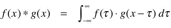
countless other tasks. Formally, for functions f(x) and g(x)
of a continuous variable x, convolution is defined as:
where * means convolution
and · means ordinary multiplication.
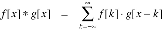
For functions of a discrete variable x, i.e. arrays of numbers,
the definition is:
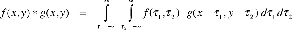
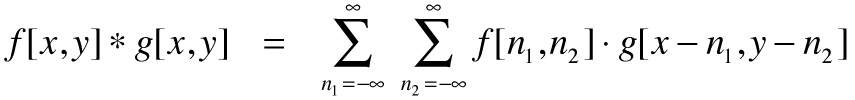
Finally, for functions of two variables x and y (for example
images), these definitions become:
and
In digital photography, the image produced by the lens is a continuous function
f(x,y), Placing an antialiasing filter in front of the sensor convolves this
image by a smoothing filter g(x,y). This is the third equation above. Once
the image has been recorded by a sensor and stored in a file, loading the file
into Photoshop and sharpening it using a filter g[x,y] is the fourth
equation.
Despite its simple definition, convolution is a difficult concept to gain an
intuition for, and the effect obtained by applying a particular filter to a
particular function is not always obvious. In this applet, we explore
convolution of continuous 1D functions (first equation) and discrete
2D functions (fourth equation).
Convolution of 1D functions
On the left side of the applet is a 1D function ("signal"). This is f. You
can draw on the function to change it, but leave it alone for now. Beneath
this is a menu of 1D filters. This is g. If you select "custom" you can also
draw on the filter function, but leave that game for later. At the bottom is
the result of convolving f by g. Click on a few of the filters. Notice that
"big rect" blurs f more than "rect", but it leaves kinks here and there.
Notice also that "gaussian" blurs less than "big rect" but doesn't leave kinks.
Both functions (f and g) are drawn as if they were functions of a continuous
variable x, so it would appear that this visualization is showing convolution
of continuous functions (first equation above). In practice the two functions
are sampled finely and represented using 1D arrays. These numbers are
connected using lines when they are drawn, giving the appearance of continuous
functions. The convolution actually being performed in the applet's script is
of two discrete functions (second equation above).
Whether we treat the convolution as continuous or discrete, its interpretation
is the same: for each position x in the output function, we shift the filter
function g left or right until it is centered at that position, we flip it
left-to-right, we multiply every point on f by the corresponding point on our
shifted g, and we add (or integrate) these products together. The
left-to-right flipping is because, for obscure reasons, the equation for
convolution is defined as g[x-k], not g[x+k] (using the 2nd
equation as an example).
An alternative way to think about convolution
If this procedure is a bit hard to wrap your head around, here's an equivalent
way to describe it that may be easier to visualize: at each position x in the
output function, we place a copy of the filter g, centered left-to-right around
that position, flipped left-to-right, and scaled up or down according to the
value of the signal f at that position. After laying down these copies, if we
add them all together at each x, we get the right answer!
To see this alternative way of understanding convolution in action, click on
"animate", then "big rect". The animation starts with the original signal f,
then places copies of the filter g at positions along f, stretching them
vertically according to the height of f at that position, then adds these
copies together to make the thick output curve. Although the animation only
shows a couple dozen copies of the filter, in reality there would need to be
one copy for every position x. In addition, for this procedure to work the sum
of copies must be divided by the area under the filter function, a processing
called normalization.
Otherwise, the output would be higher or lower than the input, rather than
simply being smoothed or sharpened. For all the filters except "custom",
normalization is performed for you just before drawing the thick output curve.
For the "custom" filter, see below.
Once you understand how this works, try the "sharpen" or "shift" filters. The
sharpen filter replaces each value of f with a weighted sum of its immediate
neighbors, but subtracting off the values of neighbors a bit further away. The
effect of these subtractions is to exaggerate features in the original signal.
The "Sharpen" filter in Photoshop does this; so do certain layers of neurons in
your retina. The shift filter replaces each value of f with a value of f taken
from a neighbor some distance to the right. (Yes, to the right, even though
the spike in the filter is on the left side. Remember that convolution flips
the filter function left-to-right before applying it.)
Finally, click on "custom" and try drawing your own filter. If the area under
your filter is more or less than 1.0, the output function will jump up or down,
respectively. To avoid this, click on "normalize". This will scale your
filter up or down until its area is exactly 1.0. By the way, if you animate
the application of your custom filter, the scaled copies will only touch the
corresponding point on the original function if your custom filter reached
y=1.0 at its x=0 position. Regardless, if your filter is normalized, the
output function will be of the right height.
Convolution of 2D functions
On the right side of the applet we extend these ideas to two-dimensional
discrete functions, in particular ordinary photographic images. The original
2D signal is at top, the 2D filter is in the middle, depicted as an array of
numbers, and the output is at the bottom. Click on the different filter
functions and observe the result. The only difference between "sharpen" and
"edges" is a change of the middle filter value from 9.00 to 8.00. However,
this change is crucial, as you can see. In particular, the sum of all non-zero
filter values in "edges" is zero. Therefore, for positions in the original
signal that are smooth (like the background), the output of the convolution is
zero (i.e. black). The filter "hand shake" approximates what happens in a
long-exposure photograph, in this case if the camera's aim wanders from
upper-left to lower-right during the exposure.
Finally, click on "identity", which sets the middle filter tap (as positions in
a filter are sometimes called) to 1.0 and the rest to 0.0. It should come as
no surprise that this merely makes a copy of the original signal. Now click on
"custom", then click on individual taps and enter new values for them. As you
enter each value, the convolution is recomputed. Try creating a smoothing
filter, or a sharpening filtering. Or starting with "identity", change the
middle tap to 0.5, or 2.0. Does the image scale down or up in intensity? The
applet is clipping outputs at 0.0 (black) and 255.0 (white), so if you try to
scale intensites up, the image will simply saturate - like a camera if your
exposure were too long. Try putting 1.0's in the upper-left corner and the
lower right corner, setting everything else to 0.0. Do you get a double image?
As with the custom 1D filter, if your filter values don't sum to 1.0, you might
need to press "normalize". Unless you're doing edge finding, in which case
they should sum to 0.0.